Why is magnetic field denoted as ‘B’?

The elegant symmetry between electric and magnetic fields was first recognized in Maxwell’s work, notably in his 1861 paper, On the Physical Lines of Force. His earliest studies on electricity and magnetism, however, date back only a few years earlier, in the 1855 article On Faraday’s Lines of Force.

In addition to identifying this symmetry, Maxwell introduced the idea of representing certain physical quantities as vector fields and established much of the notation still in use today. To a modern physicist, though, his original presentation can appear bewildering — the equations were far from tidy, initially appearing as 20 differential equations with 20 variables.

Maxwell’s equations as they appear in his textbook from 1873.

Vector quantities, including the magnetic field, were labeled alphabetically in the order they appeared.

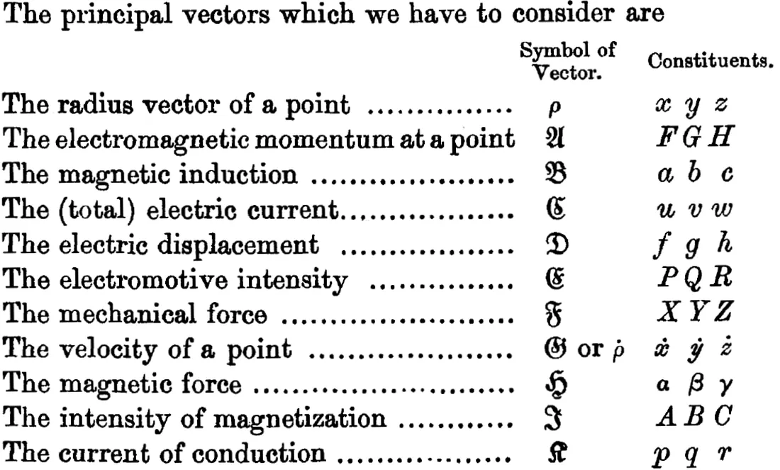
A scanned page from "A Treatise on Electricity and Magnetism", Vol. 2, p. 257.

Many of these cursive-letter labels have endured: $\mathbf{A}$ for vector potential, $\mathbf{B}$ for magnetic induction, $\mathbf{D}$ for electric displacement, $\mathbf{E}$ for the electric field, $\mathbf{F}$ for mechanical force, $\mathbf{H}$ for the magnetic field, and $\mathbf{J}$ for current. Component notation has changed (luckily!), with the electric field components evolving from $P$, $Q$, $R$ to the familiar $E_x$, $E_y$, $E_z$.

To label a magnetic field, theoretical physicists use both $\mathbf{B}=\mu_0 (\mathbf{H} + \mathbf{M})$ (magnetic induction or auxiliary field) and $\mathbf{H}$ (magnetic field) interchangeably, since in vacuum they are related only up to a vacuum permeability constant $\mu_0$.

Easter eggs from the 1873 textbook

• The table of contents includes a summary of every single page, starting the second volume with “Properties of a magnet when acted on by the earth.”

• Maxwell repeatedly discusses the necessity of the aether throughout the book.

  “Hence all these theories lead to the conception of a medium in which the propagation takes place, and if we admit this medium as an hypothesis, I think it ought to occupy a prominent place in our investigations, and that we ought to endeavour to construct a mental representation of all the details of its action, and this has been my constant aim in this treatise.”

  As is well known, the existence of the aether was finally tested in 1887. Experiments measuring the speed of light found no deviations that could account for a stationary luminiferous aether. Repeated tests confirmed this result, eventually helping Einstein establish his theory of special relativity.

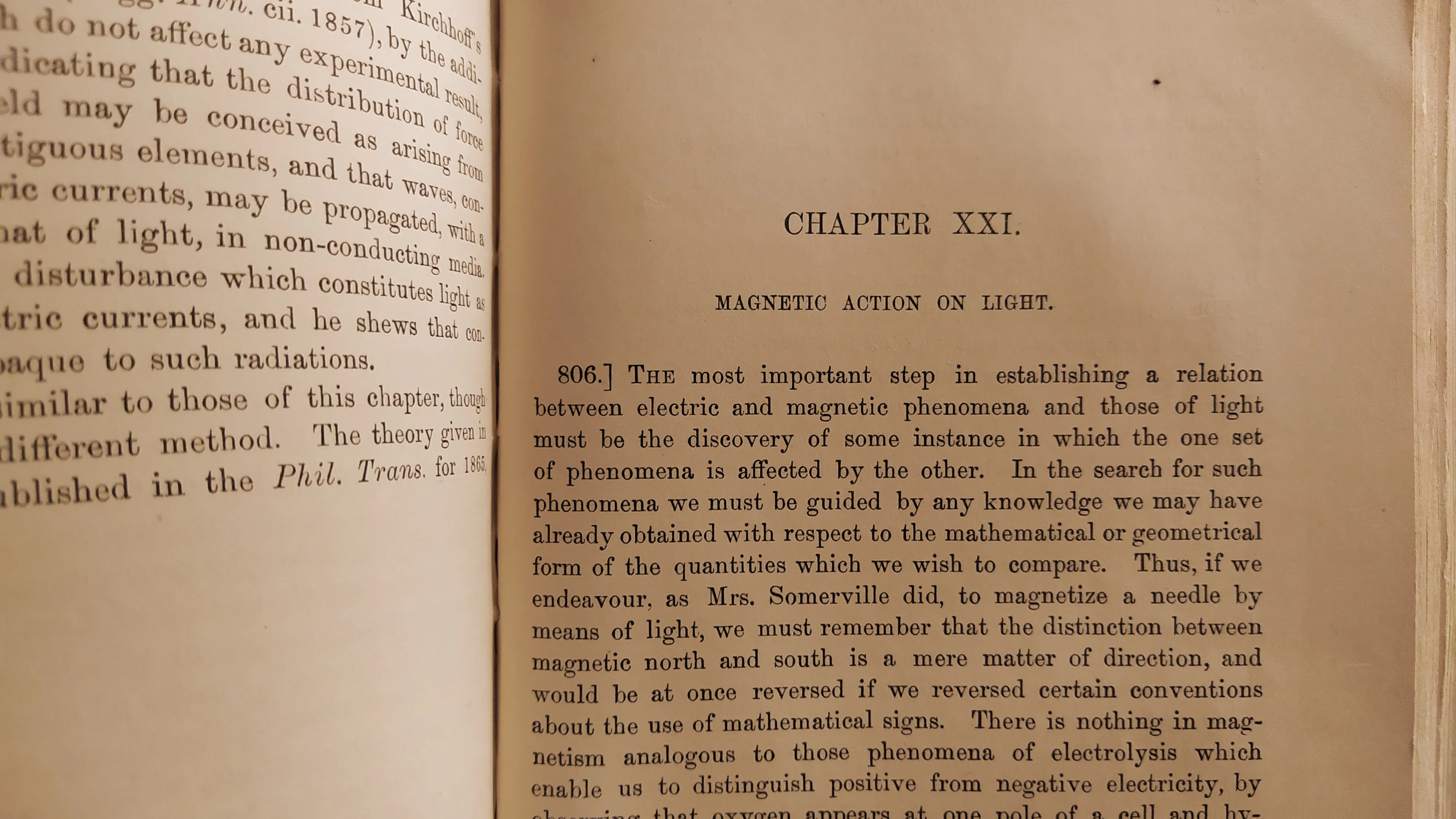
• Finally, there is this “enlightening” statement:

  “The most important step in establishing a relation between electric and magnetic phenomena and those of light must be the discovery of some instance in which the one set of phenomena is affected by the other.” [pg. 451]

Would you approve this fit?

Blunt or brilliant? You probably wouldn’t have been bold enough to fit these data like Hubble did.

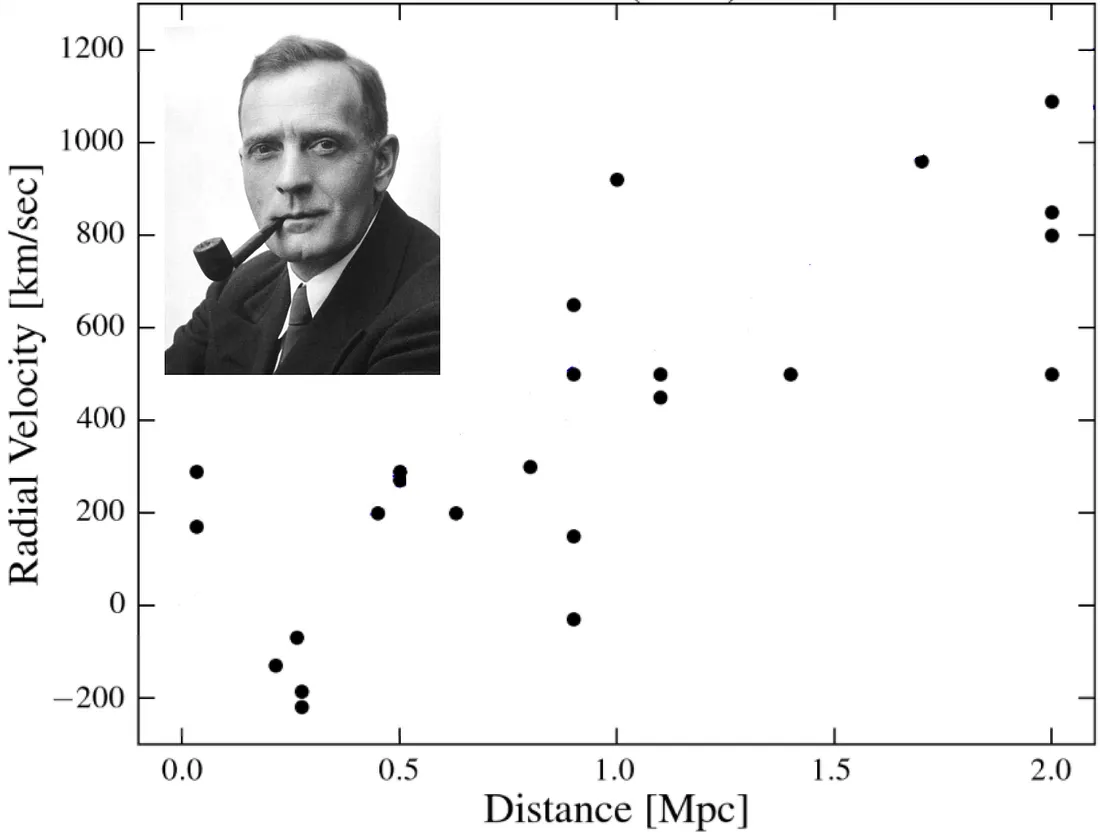
Three years before looking into these data, American astronomer Edwin Hubble concluded that among 400 objects thought of as the clouds of dust and gas and named nebulae, some were actually other galaxies. Working at Mt. Wilson’s telescope northeast of Los Angeles, he was able to distinguish the outer parts of some spiral galaxies as individual stars and found that there is more to the universe than only Milky Way. Today’s estimates suggest there are 200 billion galaxies (2×10¹¹) in the universe.

Then, in 1929, he looked into the data for measured velocities and the distances to galaxies collected in the astronomical observations. The distances to the galaxies were determined from the brightness of the stars in those galaxies. The radial velocities are corrected for the Sun’s motion, where the positive radial velocity has the meaning that the galaxy is moving away from us, while the negative means it is moving towards us.

Except for a few data points with negative radial velocity, the data (shown in the figure above) are following the trend — the farther galaxies are, the faster they are moving away from us. There were prior attempts to relate the velocity and the distance of the galaxies, but no conclusive correlation was found. From the full set of 46 data points available at the time, Hubble extracted 24 galaxies with the most reliable measurements of the velocities and distances and stated his conclusion - the correlation is linear.

Hubble’s original conclusion that the velocity vs. distance of galaxies follow the linear trend (left figure) is much more convincing from his new fit two years later (right figure), including the data from more distant galaxies (red dots).

Was he simply bold and a bit lucky, or did he also possess a deep intuition for the laws of the universe? Some view Hubble’s discovery as the most important milestone in astronomy in the 20th century because the conclusions which directly followed from it revolutionized our understanding of the universe. On the other hand, the data points which he initially fitted to the linear curve were sparse enough that this correlation he saw might be only up to chance.

Hubble’s law — the milestone in astronomy

Hubble estimated the slope in his linear fit to be 500 km/s/Mpc (kilometer per second per megaparsec), which is about 7 times greater than the best estimation of Hubble’s constant today, of about 70 km/s/Mpc. His estimation of the slope (assuming the universe was expanding with a constant rate) gives that the age of the universe is 2 billion years, less than half the age of the Earth! The biggest source of the error was in estimating the distances of the galaxies, which was fixed in the second half of the previous century when the Hubble’s constant was estimated in the range between 50 to 90 km/s/Mpc.

More importantly at the time than the number, the trend Hubble discovered, today known as Hubble’s law, made a revolution in our understanding of the universe. The correlation between the distance of the galaxies and their velocities is among the leading evidence suggesting that our universe is expanding and one of four pilar observations on which the Big Bang theory is built. Even though Hubble himself wasn’t the creator of the idea of expanding the universe, conventionally accepted understanding that our universe is static was questioned and subsequently rejected after he published his data analysis and his conclusion. When seeing Hubble’s conclusions, Einstein abandoned his work on artificially ‘fixing’ his equations of general relativity to make his model of the universe static (the attempt he later called himself his biggest blunder). The theoretical idea of the expanding universe was suggested a few years earlier. In 1922, Friedman derived this conclusion from his model of a homogenous isotropic universe. In 1927, Leimatre independently suggested some proportionality between the velocity and distance to the distant objects.

Hubble’s constant today

The value of Hubble’s constant has the meaning of the rate with which our universe is expanding, and the inverse value of Hubble’s constant gives the age of the universe if it was expanding with a constant speed.

While the traditional way to determine Hubble’s constant from the 1950s (calibrated distance ladder techniques) converged over time to the value of 73 km/s/Mpc, the new technique that started being used from the 2000s (from the cosmic microwave background radiation) converged to a different value for Hubble’s constant, 67 km/s/Mpc. Among the two measurements, the former is measuring how fast the universe is ought to be expanding from the prediction of the early universe, while the latter is measuring how fast it is expanding today as we see it. Since 2018 more techniques have been introduced, but with not small enough uncertainties to decide between the two values.

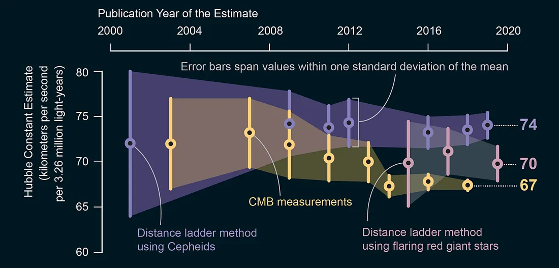
Credit: Jen Christiansen (schematics); Source: “The Carnegie-Chicago Hubble Program. VIII. An Independent Determination of the Hubble Constant Based on the Tip of the Red Giant Branch,” By Wendy L. Freedman et al., in Astrophysical Journal, Vol. 882, №1; August 29, 2019.

Although the exact value of the Hubble’s constant is important as it would give the rate with which the universe is expanding, not many astronomers or physicists were concerned with the exact number. However, the discrepancy between the two obtained values for Hubble’s constant from two different approaches becomes even stronger with new repeated measurements and is today known as the problem of Hubble’s constant.

There is actually another quantity related to the Hubble’s constant which surprised many astronomers when the discovery was made in 1998. Previously, in a famous review article from 1970, observational cosmologist Allan Sandage described the entire cosmology as a “search for two numbers,” the velocity (Hubble’s constant) and deceleration with which the universe is expanding. Then, in 1998 it was surprising to find that our universe is expanding, but with acceleration. To explain the acceleration, the Big Bang model of the universe (from Friedman equation) suggests that there has to exist dark energy, and it would account for about 75% of all mass in the universe.

Consider taking a look at Hubble’s original 1929 paper, where he discussed his findings and data fitting.

Why blue LED earned a Nobel Prize if reds and greens already existed for decades?

Red and green LEDs had been around for decades, quietly powering early electronic devices. But a bright blue LED remained elusive until 1989, when Shuji Nakamura, Hiroshi Amano, and Isamu Akasaki cracked the problem, earning them the 2014 Nobel Prize in Physics. Blue LEDs completed the RGB spectrum, making full-color LED displays and white LEDs possible. As the Nobel committee put it: “Incandescent light bulbs lit the 20th century; the 21st century will be lit by LED lamps.”

But what was so special about the blue LED that its discovery deserved a Nobel prize?

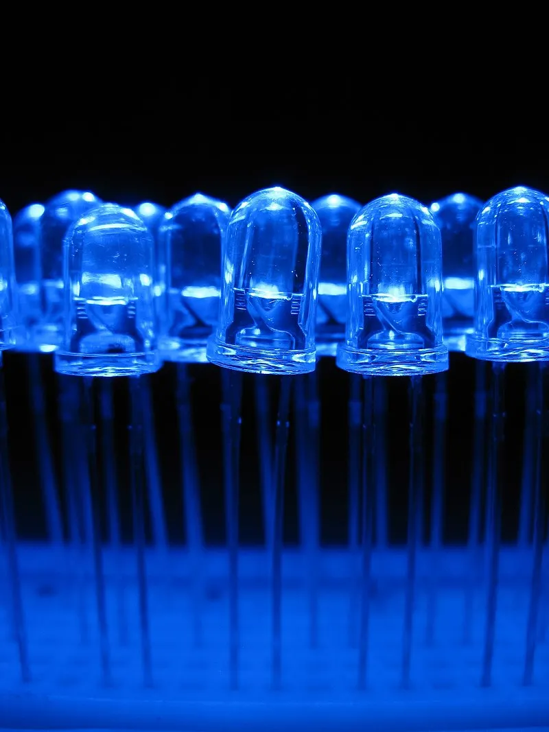
The story of the blue LED is one of perseverance, ingenuity, and a dash of luck.

A history of LEDs

A light-emitting diode (LED) is a semiconductor device that emits light when a current flows through it. The first commercially relevant semiconductor was silicon carbide (SiC). In the mid-1920s, self-educated Russian scientist Oleg Losov was the first to look deeply into the spectrum of light emission from SiC. Picking up on his work, Kurt Lehovec, Czech by birth, found in 1952 that adding different impurities and tuning their amount could change the light from blue to greenish-yellow and to pale yellow, the process now known as doping the semiconductor. A semiconductor doped with electron-rich impurities is called an n-type semiconductor, where n stands for negative charge. Similarly, a semiconductor enriched with electron-poor impurities is called a p-type semiconductor. A p–n junction is a boundary between p-type and n-type semiconductors, and an LED is a particular p-n junction that emits light.

The first infra-red LEDs at low temperatures were discovered in 1951 by a group of scientists at Bell Labs in p-n junctions of germanium and silicon. A prospective new material for emitting photons was gallium arsenide (GaAs). The first GaAs LED was discovered accidentally in 1961 by scientists working for Texas Instruments on a laser diode. It was an infra-red LED, so it had no practical use beyond the visible spectrum.

At General Electric, American engineer Nick Holonyak, Jr. was experimenting with the same material. After seeing their demonstration, he created the first visible red LED in 1962 using a compound semiconductor device combining gallium phosphide (GaP) and gallium arsenide (GaAs). He is often called the “father of the LED.” Holonyak later joined the University of Illinois, where he supervised aspiring researcher George Crawford. After completing his Ph.D., Crawford was hired by the Monsanto Company, and in 1968 Monsanto became the first to mass-produce affordable visible LEDs based on GaAs, primarily for electronic calculators, digital watches, and digital clocks.

In the mid-1970s, pure gallium phosphide (GaP) was used to make LEDs that produced green light. Another critical goal was achieving good light intensity. The first generation of super-bright red, yellow, and green LEDs came in the early 1980s. By 1987, green and red LEDs were bright enough to replace incandescent bulbs in vehicle brake lights and traffic signals, marking the first time LEDs displaced incandescent bulbs in a lighting application.

Even though color television in North America did not outsell black-and-white TVs until the early 1970s, a cathode-ray color TV was introduced in the US as early as 1953. After success with GaAs and GaP LEDs, it was expected in the late 1960s that LEDs made of gallium nitride (GaN) would emit blue light, based on nitrogen’s position in the periodic table, just above phosphorus and arsenic. The Radio Corporation of America (RCA) saw an opportunity to replace bulky cathode-ray tubes with LED-based screens. Americans James Tietjen and Herbert Maruska at RCA worked on synthesizing GaN. While producing n-type GaN became feasible, a p-type semiconductor was still needed for a functional p-n junction. With practically unlimited funding, RCA hired well-known material scientists Jacques Pankove and Edward Miller to work on blue LEDs. In 1972, RCA engineers produced a faint blue LED and patented it two years later. They had hoped these LEDs could finally complete the RGB spectrum for displays, but the light was too dim, and the financially struggling company cut funding for blue LED research in 1974. Although GaN samples had been made as early as 1969, the critical challenge of producing p-type GaN for a working p-n junction remained unsolved, leaving bright blue LEDs a tantalizing dream for decades.

Across the Pacific, Japanese engineer and physicist Isamu Akasaki began working on GaN in the late 1960s at Matsushita Research Institute Tokyo. In 1981 he joined Nagoya University and, along with his graduate student Hiroshi Amano, developed a method for p-type doping GaN. They finally produced p-type GaN and, in 1989, a p-n junction emitting high-power blue light. Engineer Shuji Nakamura at Nichia built on their work to develop a practical method for mass production. By 1993, Nakamura’s blue LEDs were 100 times brighter than previous SiC LEDs, reaching 2.7% efficiency, and became the basis for all commercial blue LEDs and laser diodes today.

The impact of blue LEDs was transformative. Today, nearly all LED devices, from smartphone screens and televisions to streetlights and car headlights, still rely on the p-n junction in GaN. Nichia remains the world’s largest supplier of LEDs.